



How many different passwords can a phone have? How likely is it that a medical test is wrong? Can a poll of 1,000 people speak for a whole country? In this chapter you will learn to count outcomes quickly, compute probabilities of combined events, work with the bell-shaped normal curve, and judge how far a survey result can be trusted.
1. The counting principle and factorials
If a task is done in stages and stage 1 can happen in \(m_1\) ways, stage 2 in \(m_2\) ways, and so on up to stage \(k\), then the whole task can be done in \(m_1\times m_2\times\cdots\times m_k\) ways.
For a whole number \(n\ge 1\), \(n!=n\times(n-1)\times\cdots\times 2\times 1\). By convention \(0!=1\). For example \(5!=120\).
A password has 3 different capital letters followed by 2 different digits. There are \(26\times25\times24\) ways to choose the letters and \(10\times 9\) ways to choose the digits, so \(26\times25\times24\times10\times9=1{,}404{,}000\) passwords.
2. Permutations and combinations
A permutation is an arrangement in which order matters. The number of ways to arrange \(r\) objects chosen from \(n\) different objects is \(P(n,r)=\dfrac{n!}{(n-r)!}\).
A combination is a selection in which order does not matter. The number of ways to choose \(r\) objects from \(n\) is \(C(n,r)=\dfrac{n!}{r!\,(n-r)!}\). Always \(C(n,r)=C(n,n-r)\).
- Ask yourself: if I swap two chosen items, do I get a different result?
- Yes (gold, silver, bronze medals): use \(P(n,r)\).
- No (a team, a hand of cards): use \(C(n,r)\).
Eight runners race. Medals for first, second and third place: \(P(8,3)=8\times7\times6=336\). Choosing 3 of the 8 runners for a relay team: \(C(8,3)=\dfrac{336}{3!}=56\).
When some objects are identical, divide by the factorial of each repeated count. The letters of BANANA (B once, A three times, N twice) can be arranged in \(\dfrac{6!}{3!\,2!}=60\) ways.
3. Independent and dependent events
Events \(A\) and \(B\) are independent when one happening does not change the probability of the other. Then \(P(A\text{ and }B)=P(A)\times P(B)\). If the second probability changes because of the first event, the events are dependent, and \(P(A\text{ and }B)=P(A)\times P(B\mid A)\).
A bag holds 5 red and 3 blue marbles. Two are drawn, and we want both red.
With replacement, the draws are independent: \(\dfrac58\times\dfrac58=\dfrac{25}{64}\).
Without replacement, the draws are dependent: \(\dfrac58\times\dfrac47=\dfrac{20}{56}=\dfrac5{14}\).
A tree diagram multiplies along each branch and adds the branches that give the same outcome. The four leaves above add up to \(\dfrac{20+15+15+6}{56}=1\).
4. Conditional probability
The probability of \(B\) given that \(A\) has occurred is \(P(B\mid A)=\dfrac{P(A\text{ and }B)}{P(A)}\), with \(P(A)>0\). Events are independent exactly when \(P(B\mid A)=P(B)\).
A two-way table makes this concrete. In a survey of 200 students, we record band membership and honor roll status.
| On honor roll | Not on honor roll | Total | |
|---|---|---|---|
| In band | 48 | 32 | 80 |
| Not in band | 42 | 78 | 120 |
| Total | 90 | 110 | 200 |
Given that a student is in band, the chance of being on the honor roll is \(P(H\mid B)=\dfrac{48}{80}=0.6\). Overall \(P(H)=\dfrac{90}{200}=0.45\). Since \(0.6\ne0.45\), the events are not independent.
\(P(B\mid A)\) and \(P(A\mid B)\) are usually different. Here \(P(B\mid H)=\dfrac{48}{90}=\dfrac{8}{15}\), not \(0.6\). Always check which group you are restricting to: it becomes the denominator.
5. Binomial distribution and the binomial theorem
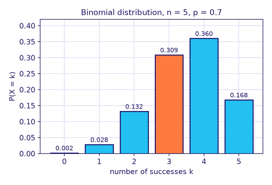
Repeat \(n\) independent trials, each with only two outcomes (success with probability \(p\), failure with probability \(1-p\)). The number of successes \(X\) satisfies \(P(X=k)=C(n,k)\,p^k(1-p)^{n-k}\). Its mean is \(np\) and its standard deviation is \(\sqrt{np(1-p)}\).
A player makes 70% of free throws. In 5 shots, \(P(X=3)=C(5,3)(0.7)^3(0.3)^2=10\times0.343\times0.09=0.3087\). The mean is \(5\times0.7=3.5\) made shots.
\((a+b)^n=\displaystyle\sum_{k=0}^{n}C(n,k)\,a^{\,n-k}b^{\,k}\). The coefficients \(C(n,k)\) are row \(n\) of Pascal’s triangle.
Row 4 is \(1,4,6,4,1\). So \((x+2)^4=x^4+4\cdot2x^3+6\cdot4x^2+4\cdot8x+16=x^4+8x^3+24x^2+32x+16\).
6. The normal distribution and the empirical rule
Many measurements (heights, fill volumes, test scores) pile up around an average and thin out symmetrically on both sides. Their graph is a bell-shaped normal curve with mean \(\mu\) and standard deviation \(\sigma\).
In a normal distribution, about 68% of the data lie within 1 standard deviation of the mean, about 95% within 2, and about 99.7% within 3.
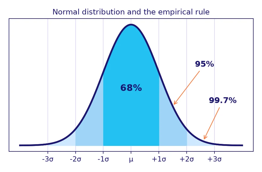
A machine fills bottles with mean 16.0 oz and standard deviation 0.2 oz. About 95% of bottles hold between \(16.0-0.4=15.6\) oz and \(16.0+0.4=16.4\) oz (about 461 mL to 485 mL). The tails are symmetric, so about \(\dfrac{100-95}{2}=2.5\%\) of bottles hold more than 16.4 oz.
7. Standard deviation and z-scores
For a data set with mean \(\bar{x}\) and \(n\) values, the population standard deviation is \(\sigma=\sqrt{\dfrac{\sum(x_i-\bar{x})^2}{n}}\). It measures the typical distance from the mean.
- Find the mean.
- Subtract the mean from each value and square the result.
- Average the squares, then take the square root.
For 4, 6, 8, 10, 12 the mean is 8. Squared deviations: \(16,4,0,4,16\), sum \(40\), so \(\sigma=\sqrt{40/5}=\sqrt8\approx2.83\).
The z-score of a value \(x\) is \(z=\dfrac{x-\mu}{\sigma}\). It tells how many standard deviations \(x\) lies above (\(z>0\)) or below (\(z<0\)) the mean, which lets you compare different scales.
On a test with \(\mu=72\) and \(\sigma=8\), a score of 84 has \(z=\dfrac{84-72}{8}=1.5\).
8. Sampling methods and bias
A population is the whole group we care about; a sample is the part we actually survey. A good sample looks like a small copy of the population.
| Method | How it works | Example |
|---|---|---|
| Simple random | Every member has an equal chance | Drawing 30 names from a hat |
| Stratified | Split into groups, sample each in proportion | 10% of every grade level |
| Cluster | Pick whole groups at random | Surveying 4 randomly chosen classrooms |
| Systematic | Take every k-th member | Every 10th person on a list |
| Convenience | Whoever is easiest to reach | Asking people at one store (biased) |
A sample is biased if some members of the population are more likely to be chosen than others. Convenience samples (asking people at a gym about exercise) and voluntary response samples (call-in polls) are usually biased, and a large sample size does not fix bias.
9. Margin of error and statistical inference
Inference means using a sample to draw a conclusion about a population. Two random samples give slightly different results, so every estimate comes with a margin of error. For a sample proportion \(\hat p\) from a random sample of size \(n\), an approximate 95% margin of error is \(ME=1.96\sqrt{\dfrac{\hat p(1-\hat p)}{n}}\), and the interval is \(\hat p\pm ME\).
In a random sample of \(n=400\) voters, 55% support a park. Then \(ME=1.96\sqrt{\dfrac{0.55\times0.45}{400}}\approx0.049\). We estimate that between about 50.1% and 59.9% of all voters support it.
On my planet we say: to cut the margin of error in half, you must survey four times as many beings. The square root of \(n\) is the boss!
Key takeaways
- Multiply the number of choices at each stage; \(n!\) counts arrangements of \(n\) different objects.
- Order matters: \(P(n,r)=\dfrac{n!}{(n-r)!}\). Order does not matter: \(C(n,r)=\dfrac{n!}{r!(n-r)!}\).
- Independent: \(P(A\text{ and }B)=P(A)P(B)\). In general \(P(A\text{ and }B)=P(A)P(B\mid A)\).
- \(P(B\mid A)=\dfrac{P(A\text{ and }B)}{P(A)}\).
- Binomial: \(P(X=k)=C(n,k)p^k(1-p)^{n-k}\), mean \(np\).
- Empirical rule: 68%, 95%, 99.7%. \(z=\dfrac{x-\mu}{\sigma}\).
- Random samples avoid bias; \(ME=1.96\sqrt{\hat p(1-\hat p)/n}\).


Test yourself: quick challenge for Grade 11
Speed drill for Grade 11: how many in 60 seconds?
🚀 Keep exploring with Zyro
 ✏️ Math practiceProbability and Statistics: math practice, Grade 11
 📝 Math testsProbability and Statistics: math test, Grade 11
 🎯 Math quizzesProbability and Statistics: math quiz, Grade 11
 ✏️ Math practiceLinear Equations, Inequalities and Systems: math practice, Grade 11
 ✏️ Math practiceQuadratic Functions and Equations: math practice, Grade 11
 📝 Math testsLinear Equations, Inequalities and Systems: math test, Grade 11